From a Research Paper to Running Code: Experimenting with Local Exploit Hazard in Vulnerability-Lookup
One of the interesting characteristics of open-source security tooling is that it gives us a relatively direct path from research to experimentation.
On 27 July 2026, Stephen Shaffer and Laura Voicu published the first version of Modeling Local Exploit Hazard — A Bayesian Framework for Quantifying Exploit Risk and Operational Efficiency on arXiv. The paper proposes turning global exploit-likelihood estimates such as EPSS into a local exploit hazard that can account for an organization’s controls, vulnerability age and exposure context.
Nine days later, on 5 August, we opened Vulnerability-Lookup PR #530 to see what would happen if we tried to implement the model in an actual open-source vulnerability-management platform rather than treating the paper purely as a theoretical exercise.
The pull request evolved considerably during the experiment and was merged on 11 August 2026 after 18 commits, touching 29 files with roughly 3,500 additions.
This article is an analysis of that experiment: what the paper proposes, which parts translate naturally into Vulnerability-Lookup, which assumptions become harder when confronted with real data and APIs, and what we learned about turning a probabilistic research model into an operational vulnerability-management feature.
Important: this is an experimental implementation of a very recent research model. The resulting hazard values should not yet be interpreted as calibrated predictions of how many security incidents an organization will actually experience.
The problem the paper tries to solve
Vulnerability-management systems have become quite good at collecting information.
For a vulnerability we can have CVSS severity, EPSS exploitation probability, KEV information, SSVC decisions, vendor advisories, sightings, exploit information and numerous other annotations.
But there remains a fundamental difference between:
“How interesting or dangerous is this vulnerability globally?”
and:
“How much exploitation risk does this vulnerability represent in my environment?”
The paper starts from this distinction.
EPSS, for example, estimates the probability that exploitation activity associated with a CVE will be observed over a forward-looking 30-day period. It is intentionally a global exploit-likelihood model. The paper proposes taking such an Exploit Likelihood Model, or ELM, and progressively localizing it using the effectiveness of security controls, the attack vector, vulnerability age and organizational exposure.
The resulting quantity is expressed as a hazard rate rather than another vulnerability score.
That seemingly small change is actually one of the most interesting aspects of the paper.
A probability is tied to a particular time window. A hazard rate can be manipulated across different time periods and, under the assumptions of the model, aggregated across multiple vulnerability instances.
The paper therefore tries to answer a much more operational question:
Given the vulnerabilities to which I am exposed, how many exploitation events should I expect, and which remediation work will reduce that exposure most efficiently?
That is much closer to the question vulnerability-management teams actually face.
From EPSS to local exploit likelihood
The first deterministic step in the model is remarkably simple.
Suppose an ELM gives vulnerability i an exploitation probability:
A security control has an estimated exploit-prevention effectiveness CE.
The remaining exploitation likelihood after that control becomes:
If multiple independent controls apply:
The important part is not the multiplication itself, but which controls are allowed to affect which vulnerabilities.
The paper aligns controls with the CVSS attack vector. A network-layer control should influence vulnerabilities with a Network attack vector, while controls protecting local exploitation should affect Local or Physical vulnerabilities instead.
PR #530 implements this directly.
A caller can provide global controls:
{
  "epss": 0.20,
  "controls": [0.5]
}
or controls specific to an attack vector:
{
  "epss": 0.20,
  "cvss_vector": "CVSS:3.1/AV:N/AC:L/PR:N/UI:N/S:U/C:H/I:H/A:H",
  "controls_by_attack_vector": {
    "network": [0.5]
  }
}
In the second example, Vulnerability-Lookup extracts AV:N from the CVSS vector and applies the network control.
An EPSS probability of 0.20 combined with a 50% effective control therefore becomes a residual likelihood of:
This deterministic portion of the model maps particularly well to Vulnerability-Lookup because EPSS and CVSS information are already associated with vulnerability records.
Where the “Bayesian” part currently stops
The title of the paper describes a Bayesian framework, but it is useful to distinguish the full framework from what PR #530 implements.
In the paper, control effectiveness is not supposed to remain an arbitrary number typed by an administrator.
Controls start from a probability distribution. Subject-matter experts provide estimates that establish an informative prior, and observations from telemetry, penetration tests, red-team exercises or Breach and Attack Simulation can update that prior through Beta-Binomial inference.
Conceptually:
This is interesting because uncertainty decreases as an organization gathers evidence about its own defenses.
PR #530 deliberately does not implement this entire measurement pipeline.
Instead, Vulnerability-Lookup accepts control effectiveness as a deterministic probability supplied by the user.
That distinction is important.
The current implementation is better described as a Bayesian-ready deterministic implementation of the downstream hazard model.
We think this is a reasonable boundary for Vulnerability-Lookup. A vulnerability database knows about vulnerabilities. It does not necessarily know whether an organization’s WAF blocked 73 out of 100 exploitation attempts, whether an EDR prevented a particular local privilege escalation, or what happened during the latest penetration test.
Those observations belong to the organization.
The API therefore creates an interesting separation: another system can estimate CE, including through the full Bayesian process proposed by the paper, and use Vulnerability-Lookup to perform the subsequent hazard calculation.
Converting probability into hazard
Once controls have been applied, the model converts the resulting probability into a hazard rate.
For a constant exponential hazard:
For EPSS, T is normally 30 days.
If a vulnerability has an adjusted 30-day exploitation probability of 0.10:
The advantage is that we can now calculate the probability over another horizon t:
PR #530 exposes this through:
POST /api/exploit-hazardThe response contains, among other values:
{
  "adjusted_likelihood": 0.1,
  "daily_hazard": 0.003512,
  "horizon_days": 7,
  "horizon_probability": 0.0243,
  "model": "exponential"
}
This already makes the model useful as an API primitive. A vulnerability-management client can ask Vulnerability-Lookup to transform its existing vulnerability intelligence into a locally parameterized exploitation estimate.
Vulnerability age and the Weibull model
The exponential model contains a fairly strong assumption: exploitation hazard remains constant with time.
A vulnerability published yesterday and the same vulnerability left unpatched for three years therefore have the same instantaneous hazard if their input ELM probability is identical.
The paper argues that this does not match observed exploitation behavior.
It therefore proposes a Weibull survival model:
where k controls how hazard changes as the vulnerability ages.
When:
k = 1, the model becomes the normal exponential model;k < 1, hazard decreases over time;k > 1, hazard increases over time.
The authors derive a default value of:
from CISA KEV timing data. They also recommend considering approximately 0.5 – 0.7 as a sensitivity range.
Importantly, the paper itself explains the limitations of this calibration: KEV addition time is not necessarily exploitation time, and CISA KEV is a curated rather than random sample.
PR #530 implements the Weibull model and uses 0.605 as its default.
For example:
{
  "vulnerability_id": "CVE-2026-XXXX",
  "controls_by_attack_vector": {
    "network": [0.5]
  },
  "model": "weibull",
  "published": "2026-07-01",
  "horizon_days": 7
}
When Vulnerability-Lookup has the vulnerability ID, the API can also obtain EPSS and CVSS information from its own metadata.
This is where the experiment starts becoming significantly more interesting than simply implementing equations from a paper.
Vulnerability age is derived from actual vulnerability records. CVSS is extracted from available metrics. EPSS comes from Vulnerability-Lookup metadata. The theoretical inputs start connecting to the datasets already maintained by the platform.
KEV: policy and probability are not the same thing
The paper contains an unusually useful discussion about KEV.
A KEV entry tells us that exploitation has been observed.
EPSS tells us something different: the probability that exploitation will be observed in a future window.
Multiplying the two as though KEV were simply another probabilistic feature is therefore not statistically clean.
The authors explicitly acknowledge this distinction but retain an optional KEV weight or floor because KEV frequently drives organizational and regulatory remediation policies.
PR #530 keeps the same separation.
A user can define:
{
  "kev_weight": 1.5,
  "kev_floor": 0.4
}
and those values are only activated when the vulnerability is actually considered KEV-listed.
The floor is applied before controls. It is therefore a policy floor on the initial likelihood, not a guarantee that the final controlled likelihood remains above that value.
This is a good example of where implementation benefits from the paper being explicit about its epistemic compromises.
KEV is retained because it matters operationally, but we should not pretend it is something that it is not.
From one vulnerability to many
A particularly useful property of hazard rates is their ability to aggregate.
The paper defines an aggregate:
and discusses using it at host, network, business-unit or organization scope.
PR #530 consequently grew beyond the original single-vulnerability API.
The merged implementation includes:
POST /api/exploit-hazard/batchwhich can evaluate multiple vulnerability instances and return both individual results and their aggregate hazard.
It also moved the model into Vulnerability-Lookup’s notification system.
The resulting implementation includes the single and batch APIs, hazard-enriched notification reports, per-subscription localization parameters and daily standing-exposure evaluation.
That evolution is perhaps the most valuable part of the experiment.
A formula is not yet a vulnerability-management feature.
A feature needs somewhere that the result affects a decision.
Hazard-aware vulnerability notifications
Vulnerability-Lookup notifications can now be enriched with the hazard calculation.
For vulnerabilities for which EPSS is available, the notification code constructs the model inputs from the vulnerability record.
When a publication date exists, it uses the Weibull model. When the age cannot be established, it falls back to the exponential model rather than inventing one.
Reports can then be ordered by descending exploitation hazard instead of merely by publication order.
This creates a practical difference.
A notification containing fifty new vulnerabilities no longer needs to present them as fifty equivalent additions. The ones contributing most to the modeled exposure can appear first.
Email, CSV and webhook reporting were extended accordingly, and subscriptions can store their own local hazard parameters.
The same public Vulnerability-Lookup instance can therefore produce different localized results for different subscribers without changing the underlying vulnerability data.
That is exactly the distinction between global vulnerability intelligence and local risk context that motivated the paper.
A worked example from the public instance
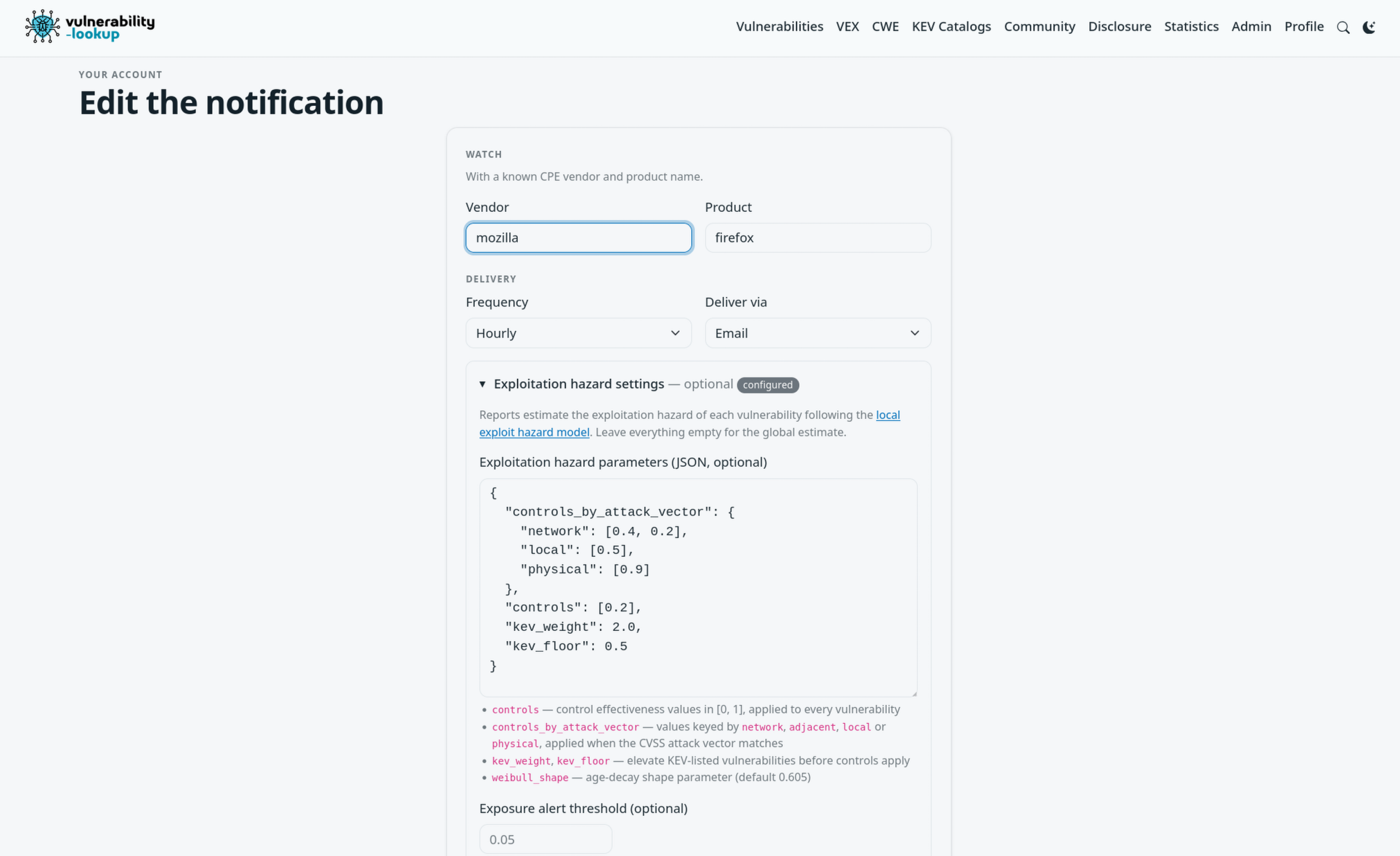
Abstract descriptions only go so far, so we configured a mozilla / firefox subscription on the public instance the way an organization running Firefox on its workstation fleet might: a secure web gateway and an extension-installation policy as network-vector controls (0.4 and 0.2), endpoint hardening for local vectors (0.5), physical access control (0.9), EDR everywhere (0.2), and a KEV policy — kev_weight: 2.0 with kev_floor: 0.5, i.e. “a known-exploited vulnerability is treated as at least coin-flip likely before our controls”. Everything not set, notably the Weibull shape, is the paper’s calibrated default.
The next hourly report opened with the batch estimate — “the 8 vulnerabilities in this report carry an estimated 0.0014 expected exploitation events per day, i.e. a 1.0% probability of at least one exploitation event within 7 days” — and put CVE-2024-9680 first:
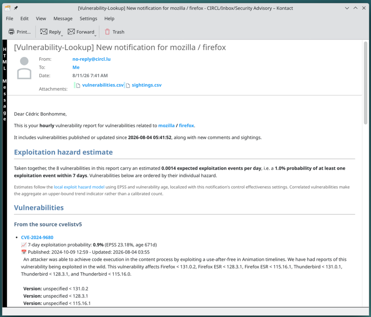
That first line — 7-day exploitation probability: 0.9% (EPSS 23.18%, age 671d) — is the whole model in one sentence, and every arrow in its derivation is one section of the paper. CVE-2024-9680 is the Firefox Animation-timeline use-after-free exploited in the wild in October 2024, so it sits in the KEV catalog. The global EPSS forecast gives it 23.18% over 30 days. The subscription’s KEV policy fires automatically: the weight doubles the likelihood to 46.4% and the floor lifts it to 50% — exploitation here is observed, not predicted. The controls then apply: it is a network-vector vulnerability, so 0.5 x 0.8 x 0.6 x 0.8 leaves a residual likelihood of 19.2%. Finally the age-conditional Weibull hazard turns that 30-day likelihood, at 671 days of age, into 0.9% for the coming week. Recomputing the same instance without the KEV flag yields 0.4% — the KEV listing alone more than doubles this vulnerability’s standing in the report.
The ranking argument then makes itself: CVE-2024-9680’s daily hazard is roughly 90% of the entire batch’s aggregate. One vulnerability carries almost all of the report’s hazard, and the ordering puts it exactly where the reader’s attention should go, above seven young entries with sub-percent EPSS scores.
A second subscription, wordpress / wordpress — parameterized as a hosting provider’s fleet — showed two further regimes of the model:
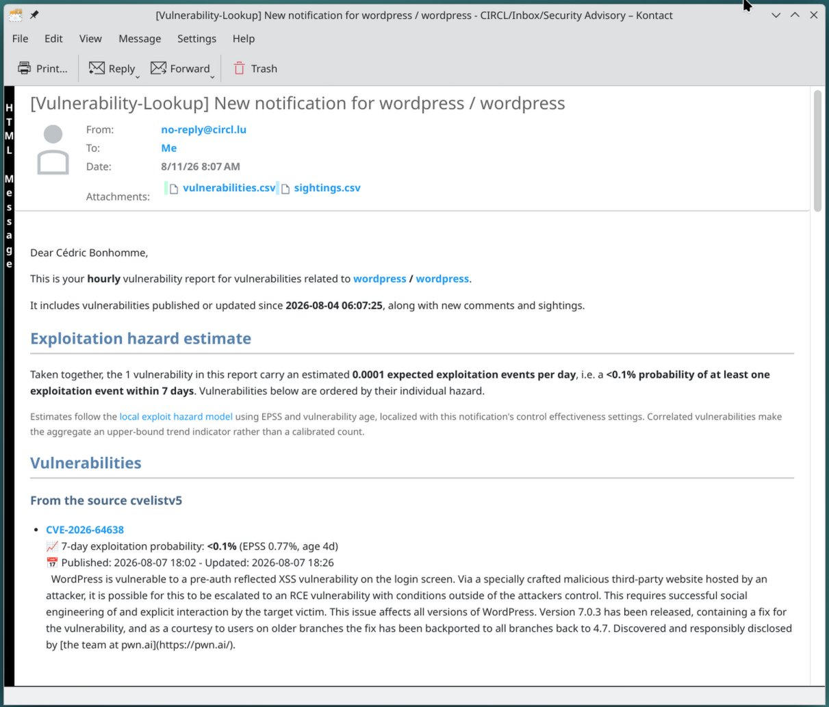
Its report carried CVE-2026-64638, a pre-auth reflected XSS on the login screen, escalatable to RCE, “affects all versions of WordPress”. The description reads alarmingly; the annotation reads <0.1% (EPSS 0.77%, age 4d). Four days after publication EPSS has barely moved, the controls cut the residual likelihood to 0.22%, and even though a four-day-old vulnerability sits near the peak of its Weibull hazard curve, the coming week works out to a 0.05% probability. The annotation resists the headline — and it is honestly a snapshot: EPSS is re-read on every evaluation, so if exploitation activity appears, the next report will say something different.
The mirror case is CVE-2022-21661, the WordPress core SQL injection from 2022, at EPSS 97.8% and KEV-listed. For it the KEV policy is a no-op — doubling 97.8% just clamps at certainty, the floor is irrelevant — because the forecast already saturates: the model treats exploitation attempts as near-certain, and the controls are the only thing standing in between. Side by side, the two KEV-listed vulnerabilities show both regimes of the paper’s KEV policy: for the under-forecast zero-day it doubles the estimate; for the saturated mass-exploited SQL injection it changes nothing — the controls do all the work.
Standing exposure instead of notification deltas
A notification normally describes change:
these vulnerabilities appeared since the previous report.
The paper asks a different question:
what is my exposure now?
PR #530 therefore adds a second concept: standing exposure.
Once per day, the notification daemon evaluates the current vulnerability set associated with a subscription and calculates its aggregate daily hazard.
Subscribers can define a threshold expressed in expected exploitation events per day.
For example:
0.05 events/daycan be read as approximately one expected event per twenty days under the assumptions of the model.
When the value crosses the threshold upward, Vulnerability-Lookup can send an alert. The threshold is re-armed only after exposure falls below 90% of the configured value, providing hysteresis rather than repeatedly alerting when a value oscillates around the boundary.
The implementation also keeps the highest-hazard contributors so that an alert can explain what is driving the aggregate rather than simply displaying one opaque number.
This starts approaching the remediation idea in the paper: identify the changes that remove the most hazard.
A captured threshold alert
We captured the full cycle on a python software foundation / cpython subscription with a threshold of 0.001 — as a policy statement, “alert me when my CPython estate exceeds one expected exploitation event per three years”. The next daily evaluation crossed it:
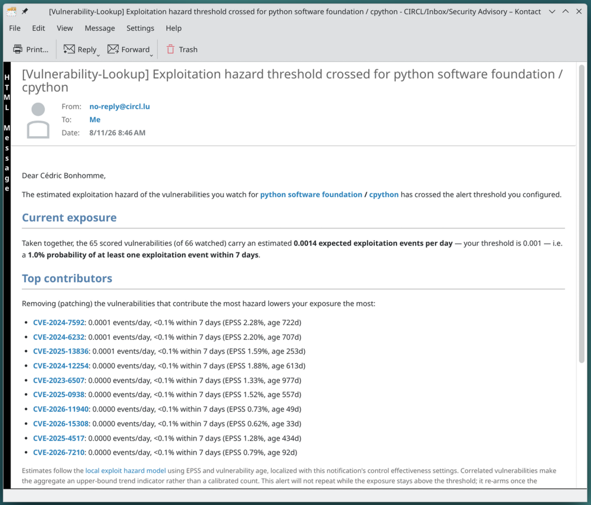
The alert reads: 65 scored vulnerabilities (of 66 watched) carry an estimated 0.0014 expected exploitation events per day — your threshold is 0.001 — i.e. a 1.0% probability of at least one exploitation event within 7 days, followed by the ranked contributors. Two details are worth noticing. First, the coverage statement (65 of 66) is part of the result: the model reports what it could not score rather than silently ignoring it — the same honesty applies to the progressive fill of very large sets, where the alert explicitly says the estimate refines on the next runs. Second, the contributor profile is the opposite of the Firefox example: CPython’s hazard is flat — EPSS scores between 0.6% and 2.3%, no KEV entry, no dominating item. The ranking is informative in both regimes: a concentrated profile (Firefox, one CVE at ~90%) points at a single patch that collapses the exposure; a flat profile says the exposure is structural and honestly low. An alert that tells you your exposure is diffuse is as much a result as one that names the patch to ship.
The delta-versus-standing contrast is also visible in production numbers: the Firefox report above carries a delta of 0.0014 events per day, while standing exposures on the public instance range from 0.02–0.18 events per day for watched sets in the low hundreds up to 1.56 events per day for one broad subscription watching 8,240 vulnerabilities. Only the standing figure answers “how exposed am I overall?”, which is why the threshold applies to it and not to the delta. And because each evaluation is stored as JSON on the notification (and carried whole in webhook alert payloads), sampling it daily yields a time series per subscription — the raw material for exactly the calibration work discussed below:
Research model versus implementation
The following table summarizes where the experiment currently stands.
| Paper concept | PR #530 | Assessment |
|---|---|---|
| ELM input such as EPSS | Implemented | Uses explicit EPSS or Vulnerability-Lookup metadata |
| Control-effectiveness adjustment | Implemented | User supplies point estimates |
| Controls aligned with CVSS attack vector | Implemented | controls_by_attack_vector |
| Bayesian SME prior | Not implemented | Expected to happen outside Vulnerability-Lookup |
| Beta-Binomial telemetry updates | Not implemented | Requires local telemetry/BAS/red-team observations |
| KEV policy weighting/floor | Implemented | Explicitly treated as policy rather than statistical evidence |
| Exponential hazard | Implemented | Direct probability-to-hazard conversion |
| Weibull age-dependent hazard | Implemented | Default k = 0.605 |
| Host aggregation | Partial | Generic vulnerability-instance aggregation, without host inventory |
| Higher-level hazard aggregation | Implemented | Batch API and notification exposure |
| Remediation ranking | Partial | Highest hazard contributors are identified |
| Grouped remediation actions | Not implemented | No patch/action simulation engine yet |
Optimization Delta (H) / Cost | Not implemented | No remediation cost model |
| Incident-frequency model | Not implemented | Paper lists this as future work |
| Financial-loss model | Not implemented | Also future work in the paper |
This distinction matters because calling the current feature a “full Bayesian implementation” would be misleading.
It implements a large and useful operational subset of the paper, but the most organization-specific Bayesian components remain external.
What does “local” mean inside Vulnerability-Lookup?
This may be the most important lesson from the experiment.
The paper’s fundamental unit is essentially an asset-vulnerability instance.
A CVE affecting 1,000 exposed servers represents something different from the same CVE existing on one isolated laboratory machine.
The paper explicitly notes that fleet size can dominate aggregate hazard.
Vulnerability-Lookup, however, is primarily a vulnerability-intelligence and vulnerability-management platform. It does not inherently know that a particular subscriber has 1,000 instances of nginx, three exposed Exchange servers and one disconnected Windows laptop.
Its notification subscriptions currently represent sets of vulnerabilities associated with vendors and products.
Consequently, the standing exposure implemented in PR #530 is currently closer to:
hazard of the watched vulnerability set
than:
hazard of the organization’s actual asset fleet.
That difference should not be hidden.
If a CVE exists on a thousand machines but appears once in the watched vulnerability set, the current aggregation does not automatically multiply its contribution by a thousand.
Conversely, many correlated CVEs affecting the same product can cause aggregation to overstate independent exposure.
So the current result is extremely useful for relative prioritization and trend analysis, but it should be treated cautiously as an absolute prediction of organization-wide exploitation-event frequency.
This is exactly the kind of difference that only becomes obvious when trying to put a research model into a real application.
The independence problem
Both the paper and implementation rely on independence assumptions.
Controls are combined as though their prevention probabilities were independent.
Vulnerability hazards are aggregated under similar assumptions.
In reality, security controls are often correlated.
A reverse proxy and WAF may share configuration. Multiple EDR controls may depend on the same telemetry. Several CVEs may affect the same software component. A campaign may exploit hundreds of systems through one common vulnerable gateway.
The paper explicitly discusses this limitation and suggests component-level grouping and, eventually, graph-based dependency modeling as future refinements.
For Vulnerability-Lookup, this means should currently be treated as a model output with assumptions, not a ground-truth counter.
The fact that the implementation and documentation expose that limitation is important.
A mathematical follow-up: integrating the Weibull aggregate
Implementing the paper also uncovered one concrete point that deserves a follow-up change.
For an exponential model, the hazard is constant, so the cumulative hazard over T days is simply:
The current aggregate implementation therefore calculates:
expected_events = aggregate_daily_hazard * horizon_days
probability_at_least_one_event = 1 - exp(-expected_events)
This is exact for the exponential model.
It is not exact for the Weibull model, because Weibull hazard changes over the horizon.
The paper gives the conditional exploitation probability for a vulnerability currently aged t:
The corresponding cumulative hazard is therefore:
The implementation already calculates the correct per-vulnerability horizon_probability.
But when building the aggregate, it currently takes the instantaneous daily_hazard and multiplies it by the number of days.
For k < 1 hazard is declining, so this tends to overestimate the forward cumulative hazard, particularly for young vulnerabilities.
With the default k = 0.605, for example, using the instantaneous hazard of a one-day-old vulnerability across the following seven days produces roughly 1.68 times the exact integrated cumulative hazard. At 30 days of age the difference falls to roughly 4%, and by 90 days it is around 1.5%.
So this matters most exactly where the Weibull model is supposed to matter most: newly disclosed vulnerabilities.
A straightforward improvement would be to aggregate cumulative hazards instead:
cumulative_hazard = sum(
    -log1p(-result["horizon_probability"])
    for result in results
)

expected_events = cumulative_hazard
probability_at_least_one_event = 1 - exp(-cumulative_hazard)
This has another useful property: it works for exponential, Weibull and even mixtures of both.
The instantaneous:
aggregate_daily_hazardcan remain useful as the current exposure rate and as an alert threshold. But a forward-looking expected_events value should integrate the hazard over the requested period as described by the paper.
This is a good example of why implementing research is useful even when the implementation is imperfect: code forces ambiguous mathematical assumptions to become explicit.
Another open question: are we applying age twice?
There is also a research question worth investigating empirically.
Vulnerability-Lookup obtains a contemporary ELM probability such as today’s EPSS value and then applies an explicit Weibull age-decay function.
This makes sense if the ELM probability is essentially age-neutral.
But if an ELM already incorporates temporal information, vulnerability maturity or signals strongly correlated with vulnerability age, an additional Weibull decay could partially count the same phenomenon twice.
This does not mean the approach is wrong.
It means it needs calibration.
One of the advantages of having the model implemented in open source is precisely that we can now compare predictions produced by:
EPSS
EPSS + controls
EPSS + Weibull
EPSS + controls + Weibull
against future observations.
The model should ultimately earn confidence through calibration, not simply because its equations are elegant.
The KEV-derived Weibull shape also deserves continued testing
The default k = 0.605 is useful because it gives us something concrete to experiment with.
But it should not become a new magical security constant.
The paper derives it from time between vulnerability publication and CISA KEV addition. The authors correctly note two major sources of bias: KEV inclusion can happen after exploitation actually began, and CISA’s catalog represents a selected population of vulnerabilities rather than a random exploitation sample.
PR #530 therefore makes the shape configurable.
That is the right engineering choice.
Different ecosystems, product classes and exploitation environments may eventually justify different age functions.
One interesting future direction would be deriving and comparing Weibull parameters from several exploitation/sighting datasets rather than treating one KEV catalog as universally representative.
The less glamorous part of research-to-production: input validation
The equations were not actually the most difficult part of the pull request.
A public API needs to survive arbitrary input.
Early reviews found cases involving negative time horizons, infinite floating-point values, malformed JSON, incorrect field types and ambiguous parsing.
For example, an early exponential calculation could produce a negative horizon probability from a negative horizon, while values approaching probability 1 could lead to non-finite numbers unsuitable for JSON.
Subsequent reviews also examined non-string CVSS vectors, date parsing, boolean handling and other cases where seemingly harmless Python coercion could transform bad API input into a server error.
The final implementation consequently contains explicit probability validation, finite-number checking, limits on control arrays, bounded time values, shape bounds, stricter ISO date handling and explicit JSON errors.
This is another useful lesson from the experiment.
A research paper might need six equations.
A usable public implementation needs those equations plus hundreds of lines dealing with everything that happens around them.
Operational scalability matters too
Standing exposure creates a second engineering problem.
An organization may watch tens of thousands of vulnerabilities, while EPSS values change every day.
Re-parsing every vulnerability record for every subscription on every evaluation would be unnecessarily expensive.
The implementation therefore separates rapidly changing data from mostly static data.
EPSS is fetched fresh during each exposure evaluation. CVSS vectors and publication dates are cached because they change much less frequently. Storage operations are pipelined, cache misses are filled under a per-run budget, and subscriptions sharing the same watched vulnerability set and hazard parameters can reuse computations.
This part has almost nothing to do with Bayesian inference or survival analysis.
But it has everything to do with whether the research can actually run continuously inside an operational open-source platform.
Remediation: the most interesting part still ahead
The paper eventually moves beyond calculating risk.
For a proposed action a, it compares current aggregate hazard H_0 with the hazard after that action H_a:
Candidate actions can then be ranked by hazard removed.
If remediation cost c_a is known:
provides an estimate of hazard reduction per unit of remediation effort.
This is potentially much more interesting than another vulnerability score.
PR #530 currently approximates the first step by retaining the vulnerabilities making the largest individual contributions to the standing hazard.
For independent single-vulnerability removal, this is effectively the right direction: removing the largest contributor removes the most hazard.
But real remediation actions do not map one-to-one to CVEs.
One operating-system update might fix forty vulnerabilities. An nginx upgrade might remove five CVEs from 2,000 servers. A firewall rule might simultaneously reduce exploitation likelihood for hundreds of vulnerabilities.
A future implementation could therefore introduce explicit remediation actions containing sets of affected vulnerability instances and optional effort estimates.
That would move Vulnerability-Lookup much closer to the remediation-ranking part of the paper.
What we would explore next
The experiment suggests a fairly natural progression:
- Correct forward aggregate calculations for non-constant Weibull hazard by summing cumulative hazard rather than multiplying instantaneous hazard by the time window.
- Clearly distinguish vulnerability-set hazard from asset-instance hazard in APIs and user interfaces.
- Allow external asset-management systems to supply real asset-vulnerability instances, perhaps including multiplicity, exposure and control-profile information.
- Add explicit remediation-action simulation so a patch, upgrade or mitigation can be evaluated as one operation rather than as independent CVEs.
- Add remediation effort or cost and calculate
Delta (H) / Cost. - Experiment with Beta control-effectiveness distributions and propagate their uncertainty rather than accepting only point estimates.
- Validate predicted hazard against subsequent exploitation observations and sightings.
- Compare different Weibull calibrations and determine whether one global age-decay parameter is actually defensible.
- Eventually investigate correlated vulnerabilities, shared infrastructure and graph-based exposure rather than relying exclusively on independence.
These would transform the current deterministic implementation into something much closer to the complete framework proposed by Shaffer and Voicu.
Why this experiment matters
PR #530 is useful even if we eventually change significant parts of the implementation.
Actually implementing the paper exposed several questions that are easy to overlook while reading it.
What exactly constitutes an “instance”?
Where does control-effectiveness data come from?
Is EPSS a probability that can safely be applied independently to every vulnerable host?
Are vulnerabilities independent enough to add their hazards?
Does an age model duplicate information already present in the exploit-likelihood model?
Is KEV part of probability estimation or remediation policy?
What does “0.05 exploitation events per day” mean when the input is a list of unique CVEs rather than a real asset inventory?
And what should happen when the mathematically elegant input is NaN, -3 days or malformed JSON?
Those questions are not arguments against the research.
They are the reason implementing research in real open-source software is valuable.
The paper provides a compelling way to move vulnerability prioritization away from static severity scores and toward a quantity with useful temporal and aggregation properties. Vulnerability-Lookup provides the vulnerability intelligence, APIs and operational workflows needed to test whether those ideas remain useful when confronted with actual data.
PR #530 is therefore better considered the beginning of an experiment than the final implementation of a new risk metric.
The most promising result is probably not the new /api/exploit-hazard endpoint itself.
It is that we now have an open implementation against which assumptions can be tested, numbers can be calibrated, alternative models can be compared and the research can be challenged with real vulnerability-management data.
That feedback loop between research, open data and open-source implementation is exactly what we wanted to explore.
References
Research paper
Stephen Shaffer and Laura Voicu, Modeling Local Exploit Hazard — A Bayesian Framework for Quantifying Exploit Risk and Operational Efficiency, arXiv:2607.24618v1, 27 July 2026.
Vulnerability-Lookup implementation
Vulnerability-Lookup PR #530, Add local exploit hazard API.
Funding
Vulnerability-Lookup is co-funded by CIRCL and by the European Union under FETTA (Federated European Team for Threat Analysis) project.